Understanding SPL metric “dB C Minus A”
When measuring SPL, indicating the frequency weighting curve used for the measurement is critical. Below we see the A (orange) and C (red) weighting curves, the two choices you are likely to encounter on a typical SPL meter, thanks to IEC 61672.
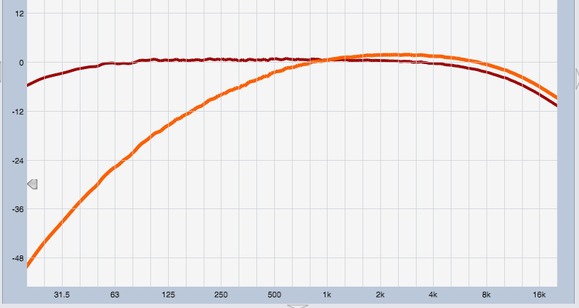
Orange = A weighting
Although these weighting curves owe their creation to a failed attempt at emulating human tonal perception at various SPLs, the focus of this discussion is their remarkable difference in the low frequency range. While the C curve extends all the way to the lower limits of human hearing with only a slight rolloff, the A curve has a significant LF rolloff, hitting about -20 dB by 100 Hz. In practical terms, the subwoofer range is virtually ignored. (As an aside, this highlights the ineffectiveness of using A-Weighted measurements to evaluate nuisance noise complaints, as most current legislation specifies, therefore completely ignoring the most commonly problematic frequency range.)
So the rule of thumb for SPL measurements is to use C Weighting if you want your measurement to include the sub range, and use A Weighting if you don’t. (A Weighting is widely used for sound exposure measurements because it tends to correlate well with noise-induced hearing loss, a topic covered in this post.)
The focus here is the additional information to be gained by looking at both C and A Weighted data together. (With apologies to Tolkien, there is no one metric to rule them all. Viewing multiple gives us much more context.)
If C levels are significantly higher than A levels, we know that there’s a lot of energy concentrated in the lower frequency range, where the A scale isn’t sensitive to it. If the readings are similar in level, that tells us that most of the energy is higher up in the frequency range.
Let’s see an actual example:
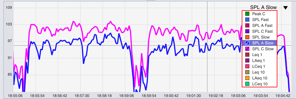
Here we have two songs from a small outdoor concert I mixed back in the summer of 2019, viewing SPL C Slow and SPL A slow. We can see the C Weighted levels are pretty steadily about 4 to 5 dB higher than the A Weighted levels. To clarify the data, let’s look at Leq 1 and Leq 10:
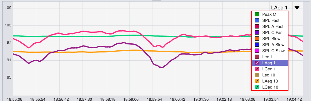
Throughout this time range, the average level for the C-Weighted data (L50) is 5.3 dB higher than the L50 for the A-Weighted data. In other words, C-A = 5.3 dB. (And, as a note, this is a relative value, comparing two dB SPL values, so the unit is dB, not dB SPL.)
Although it’s good practice to include a time specifier (Fast, Slow, Leq 1, etc), in most cases the C-A value stays pretty consistent, within about a dB, regardless of the time window we look at (because both measurements are using the same time integration).
In simple terms, the C-A metric is sort of a one-number indicator of the amount of “tilt,” or how much of the signal’s energy is concentrated in the LF region. This makes it a remarkably useful metric for show-to-show mix consistency, especially when dealing with a different room and PA system each night.
C-A also plays a role in sound exposure and noise pollution applications. A Weighted SPL is generally a good indicator for noise-induced hearing loss, although extremely high levels of low frequency energy can be damaging, so if a mix has a high C-A value, that is a good indicator that additional attention should be paid to LF exposure. (This is detailed in the AES Technical Group paper regarding sound exposure and noise pollution, available here, to which I was a contributor.)
Smaart currently calculates a Leq1 C-A as a logfile metric, but due to its usefulness as both a mixing tool and for health and 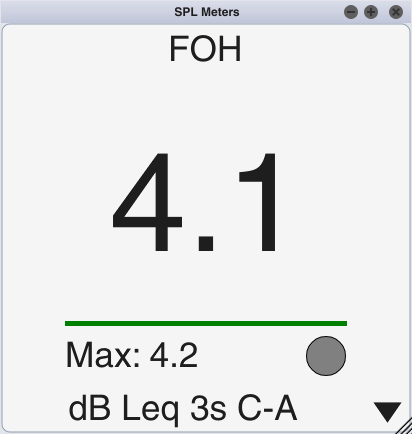 safety considerations, update v8.5 will add “C-A” as a weighting curve option for Leq measurements, which makes it available as realtime data both in the SPL History Timeline and on a meter.
In the process of testing this feature, I have found Leq 1 C-A to be a very useful metric overall, with a shorter term Leq 3s C-A behaving very similarly to an “SPL Slow” type of meter ballistic, which is helpful for studying short sections of music. It should be noted that the average (L50) of both metrics tend to closely agree over longer periods of time.
A few experimentally-determined observations:
- Pink noise extending from 20 Hz to 20 kHz has a C-A of just less than 2 dB.
- Recorded music tends to have a C-A of about 4 to 5 dB, which is relatively consistent over genre, with outliers being some jazz and orchestral music, which had a C-A of about 1 to 2 dB in my tests.
- Live music tends to have a C-A of about 8 dB, but this varies a bit as well. Using data from 14 concerts I metered during 2019, the mean C-A was 8.6 dB, with a standard deviation of 2.2 dB. This squares with our expectation that live music generally has more LF energy than recorded music.
- We are used to thinking of a 10 dB increase as perceptually about “twice as loud” but a closer look at the Equal Loudness Contours reveals that, in the LF region, the Contours are very closely packed vertically. This tells us that in the subwoofer range, about a 5 dB increase in SPL results in a 10 phon increase, which represents a doubling of perceived loudness. Therefore, the LF range during a typical live concert could be considered more than twice as much subbass to a typical listener when compared to a typical album mix played at the same level.
However, we can’t fall into the trap of simply thinking about C-A as “sub energy indicator.” For example, in this bluegrass song, the C-A value continuously decreases as the song progresses.
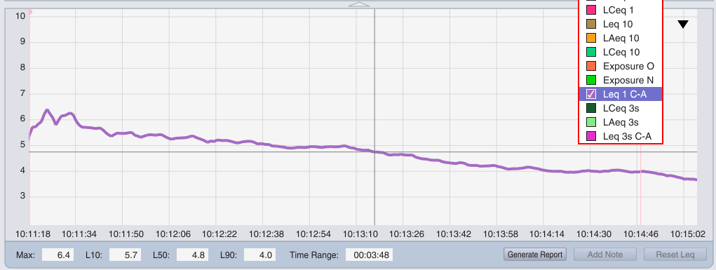
This doesn’t mean the LF energy is decreasing as the song goes on! In fact, it remains relatively consistent throughout. What’s really going on here is that the A-weighted level is increasing due to the more extensive 3-part vocal harmonies towards the end of the song. That’s more hi-mid / HF content towards the end, which changes the overall distribution of energy in the frequency spectrum more towards the HF.
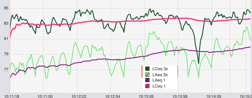
Viewing the C- and A-Weighted Leq 3s data reveals the trend:
So a safer way to think about C-A might be an indicator of how much of the overall energy resides in the subwoofer range, beyond the reaches of the A-weighting curve.