This article is the first in a two-part series that examines basic beamsteering in the context of modern sound systems.

Part one (you are here) will explain the fundamental concept of using time delay and phase offset between array elements to affect directivity, and the associated effects in the time domain.

Part two will then explore how these principles are employed by three major loudspeaker manufacturers in under-the-hood processing to achieve the desired result, and look at the practical pros and cons of each approach, and of electronic beamsteering as a whole. 

Meet the Players

To illustrate the fundamental mechanism at play, let’s look at a line of subwoofers spaced by 3 feet (between acoustic centers, not between cabinets). Let’s view their behavior at 63 Hz:

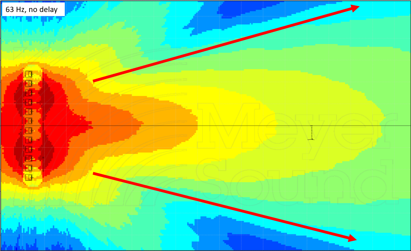
This is a coverage shape that mixers affectionately refer to as Power Alley. In front, the arrivals from all 12 elements are very close in time, and so sum together quite well. Once we get into the “blue rivers” off to either side, we have moved far enough away from center that we now have significant time offset between arrivals, and the staggered arrival times start to create a cancellation. I have added red arrows to indicate the approximate coverage angle of this array. 

The astute observer will notice a “gull wing” side lobe forming even further off axis – over here, the time offset between element arrivals has increased even further, to the point that the more distant boxes are starting to end up a full cycle behind the closer ones – they are getting “lapped” – and so starting to sum again (they are in phase, but not in time). Considering that a full cycle at 63 Hz is about 16 ms, it makes sense given the length of the line that we would have the late arrivals showing up 16 ms behind the early ones. 

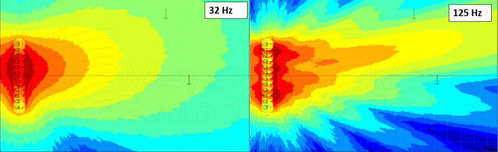
It’s also important to extrapolate based on this information that we get a different pattern at different frequencies. For example, if we view the same prediction at 125 Hz (an octave up):

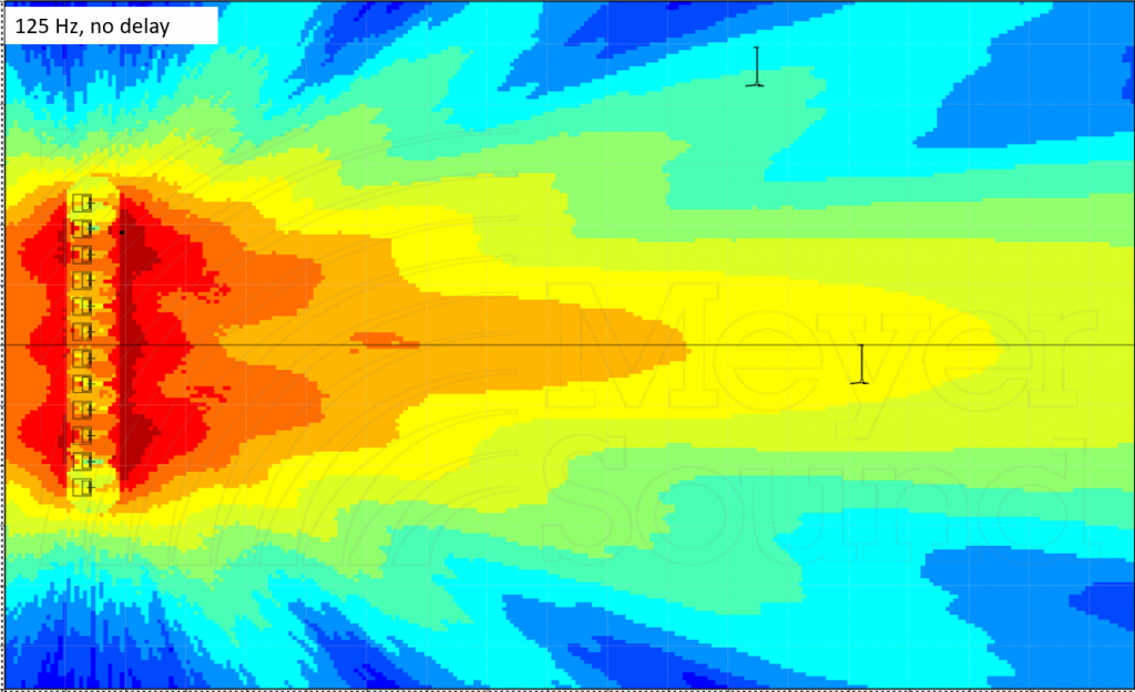
The main coverage angle has narrowed by about half. This makes sense – 125 Hz has a period of 8ms, which is half of the period of 63 Hz, and so as we start to move off axis, we only need to go half as far to accumulate enough time offset for our summation to break down. 

This idea ends up becoming one of the most important concepts in the discussion to come: a given amount of time offset (delay) will cause different amounts of phase offset at different frequencies. 

Given the narrow bandwidth of subwoofers (practically speaking, about 2.5 octaves) we have a little more leeway when using delay to steer the coverage, but this is a luxury we will not be afforded when we move to full range sources (8 octaves). The “right” amount of delay to accomplish our desired steering at a certain frequency will be ineffective lower in frequency, and create disastrous amounts of phase offset a few octaves up. 

Another concept that is important to note before we move forward: a single subwoofer is, more or less, omnidirectional at 63 Hz. When we start arraying them together, their coverage patterns all overlap significantly, and it’s this overlap that creates the beam narrowing (power alley). Manipulating the coverage pattern electronically, i.e.  by playing with timing / phase offsets between elements – is only effective if those elements have overlapped coverage such that they can interact with each other. This is a safe bet at 63 Hz, but less so at 4 kHz with a modern line array element, which exhibits very narrow vertical coverage in the high frequency range. So we need overlap to make this work. 

Another way of thinking about this: within the LF range where the elements are highly overlapped, line length is what determines the resulting coverage angle. The reason the coverage is half as wide an octave up is that the line length is doubled when viewed as a function of frequency. In other words, our subwoofer line is approximately 2 wavelengths long at 63 Hz, and approximately 4 wavelengths long at 125.

If we made the line longer such that it was now 4 wavelengths long at 63 Hz, we’d see the same coverage angle that we’re seeing now at 125 Hz (Figure 2), and 32 Hz would be making the same coverage angle that 63 is in Figure 1. 

Going forward, successful beam steering with full-range sources will rely upon finding a mechanism that allows us to affect the time / phase offsets between sources in the frequency range we want to steer, without disturbing the timing / phase relationships at other frequencies. In other words we will need frequency-dependent processing of some sort. 

Beam Spread

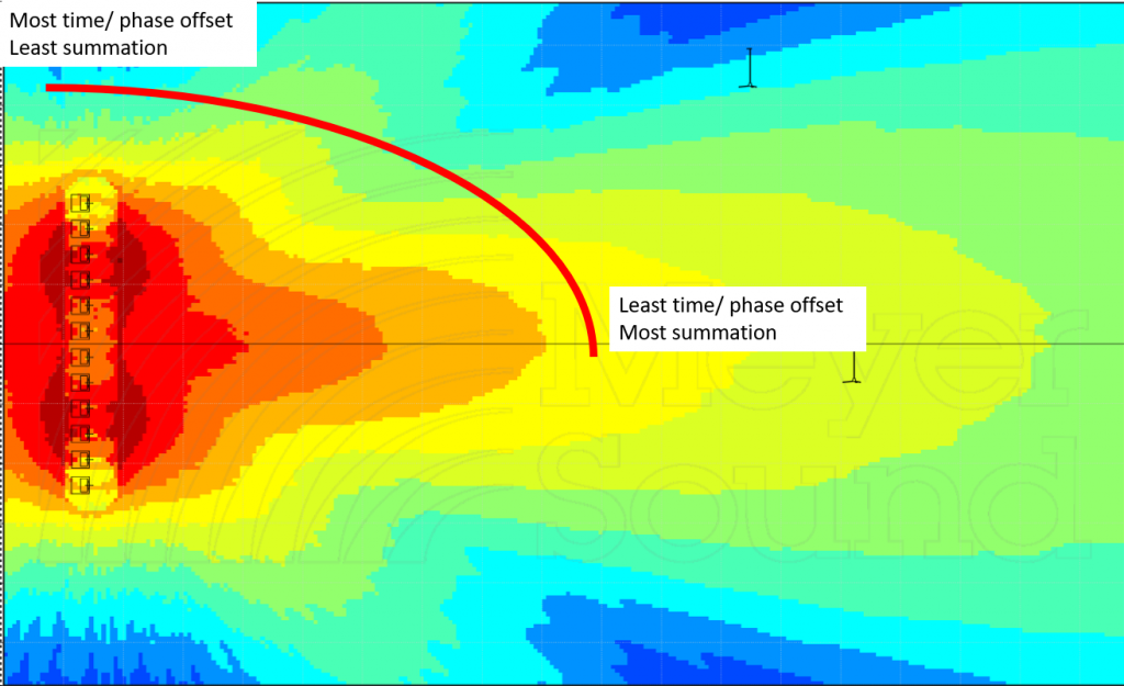
Conceptually, we have a situation where our sources are effectively omnidirectional, so they all have a similar level regardless of where we choose to stand. The difference in arrival time is the major player in determining the combined coverage shape. Without any delay in the sub array, all the arrivals are in time out in front (‘on axis’) and time offset (and therefore phase offset) accrue as we move radially to the side. Grab a laser disto, stand out in front of the array and measure the distance from your position to each element in the array. The numbers will all be similar. Now stand 90° off to the side (at the end of the line) and repeat the experiment – a much larger variance in distance, which means much more time offset.

Geometrically speaking, the time offset is least out in front, which is why we have the most summation there (power alley), and it is most on the sides of the array, where the cancellation is strongest. 

Simply: least time offset in front, most time offset on the sides. 

We can disrupt this interaction a bit by adding progressively more delay to elements that are further from the center of the array. Now they are not all arriving quite so close in time out in front – we have staggered the arrivals a little bit more, which should break down the summation a bit. Similarly, as we move off axis, the elements on the ends of the line won’t be quite as early to the party as they were before – because we delayed them. So by adding a delay taper towards the ends of the array, we increase time offset in the front, and decrease time offset on the sides.

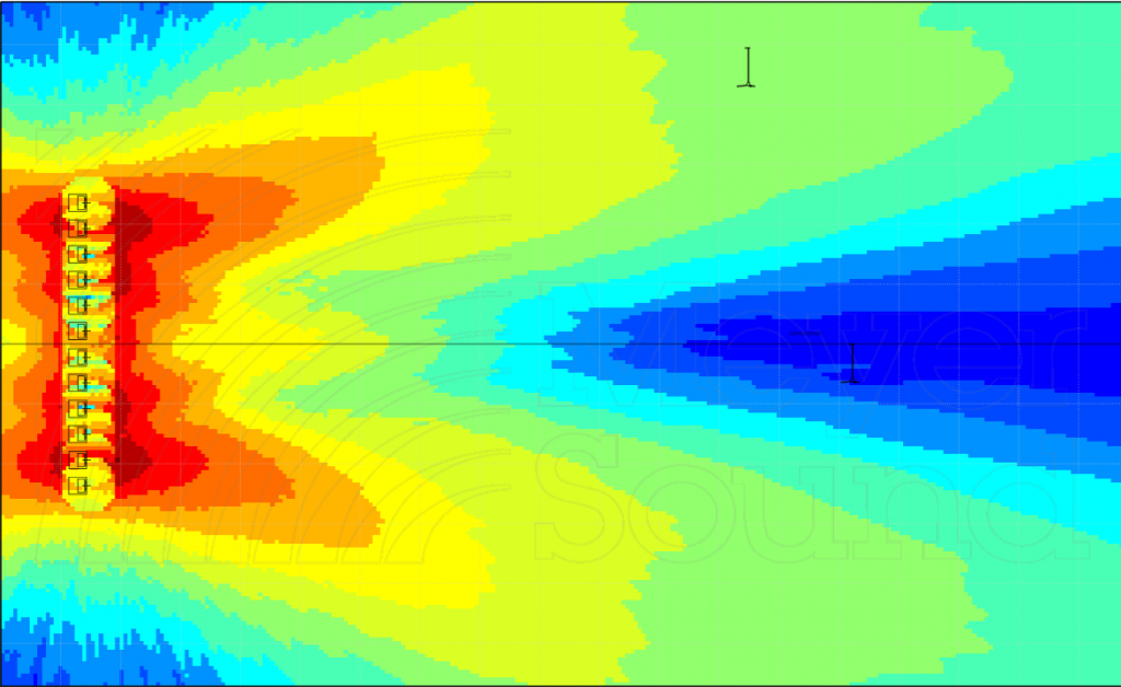
Let’s try this with a 1ms linear taper. We’ll leave the center pair at 0 ms, add 1 ms of delay to the next pair, 2 to the next, and so forth, until the outermost pair has 5 ms. 

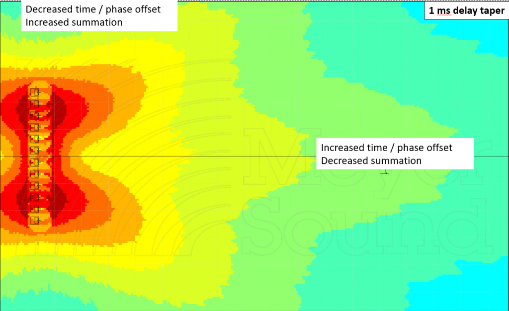
This has the desired result: widening out the coverage angle (compare to figure one) and keeping things more radially consistent (less level drop as we move off towards the sides of the array). This is helpful.

However, it’s not free. Let’s look at what’s happening at 125 Hz:

We have too much of a good thing. The time offsets that were helpful at 63 Hz are too much at 125 Hz, because they create twice as much phase offset out in front, resulting in a cancellation going forward. If we want to find a way to make this steering work with full range systems, we will need to find a way to adjust time / phase offset per frequency. 

Impulse Response

Before we move on, let’s take a second to examine the time domain ramifications of what we’re doing. By staggering the arrival times of elements out front, we have energy from the sub array arriving over a longer period of time at mix position.

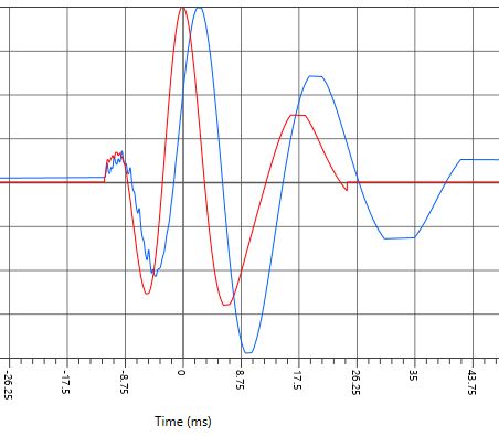
The peak in the IR is a bit later in time for the delay-tapered array (blue) compared to the non-steered array (red), which makes sense, as more of the energy is arriving later, and also the overall impulse response is lengthened by more than 15 milliseconds. This can be referred to as ‘time smearing’ and is sometimes described by FOH mix engineers as “pillowy” or “squishy”, which seem to be subjective descriptors of the fact that the impulse response of the subwoofer array is longer, and less “sharp” or “tight.”

As a practical note, gathering clear impulse response data at these low frequencies is extremely challenging in a real-world acoustic environment, a topic that we’ll be revisiting later in this series. Fortunately, the MAPP XT prediction is helpful in this regard. (Note: As of writing, the other two prediction software platforms we will be using for this series do not offer the ability to view impulse response, although I have submitted feature requests for such.)

By the way – what do you think is happening to the IR of the sub array over off to the sides, where the blue rivers were in Figure 1? The opposite – the blue river was caused by staggered arrivals over time, and our delay tapering has made them “less staggered”. The blue rivers filling in mean less time-domain stagger and a tightening of the IR. 

Steer Up

Now let’s try a variation on the same thing. Instead of applying delay from the center outward, let’s start one end at 0 ms and apply progressively more delay in 0.5 ms steps as we move to the other end, ending up at 5.5 ms on the last element.

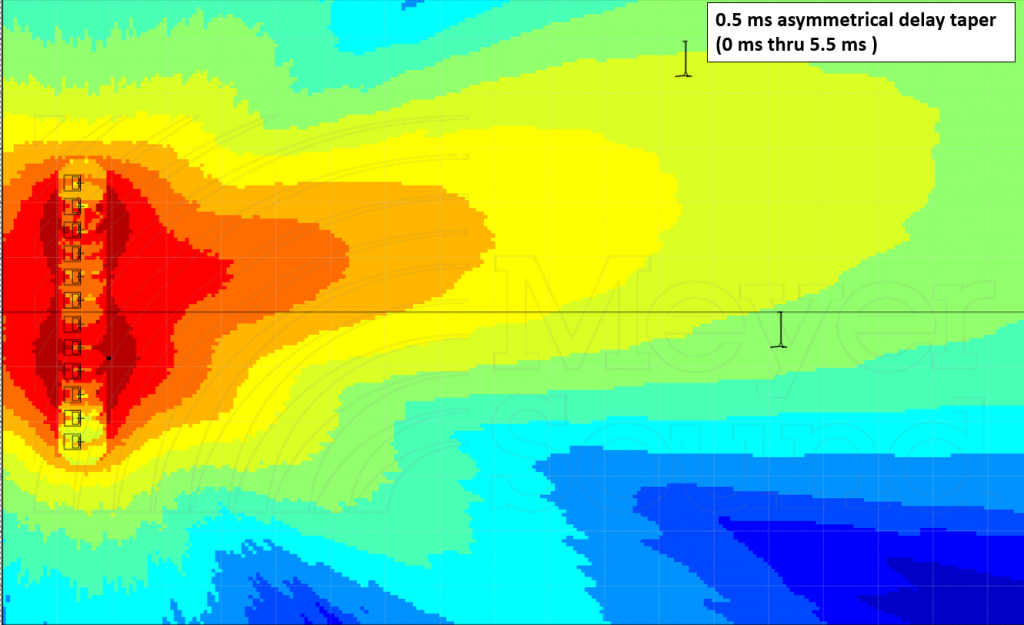
The element closest to the bottom of the image has no delay, and the element closest to the top has the most. Remember what caused power alley – equal-level, equal time. We haven’t changed levels, but we have changed where “equal time” is in the space, and moved it closer to the top of the image by giving the boxes lower down a head start. In effect, we have pointed power alley in a different direction. 

Remember that the frequency-dependent effects still hold true: coverage will still be wider at 32 Hz and narrower at 125 Hs, and that’s a limitation of relative line length and using frequency-independent delay. 

Now that we’ve look at the basic concepts, the next article we’ll learn how manufacturers are putting them to work in beamsteering algorithms.