Understanding 2-Element Cardioid Subwoofer Arrays
Thanks to the proliferation of powered loudspeakers, active subwoofers sporting built-in “cardioid mode” DSP settings are on the rise. But what’s going on under the hood?
Let’s take a look at the principles behind cardioid subwoofer arrays, clear up common confusions, and learn how to deploy these arrays in the field.
Before digging into how to steer subwoofer coverage, let’s ask why we might want to do that. Unlike full-range loudspeakers, we can’t simply aim subwoofers in the direction we want the sound to go. It’s often repeated that subwoofers are omnidirectional, dispersing their acoustic energy in all directions. Throughout the frequency range in question, the wavelengths are so long (over 37 feet at 30 Hz) that the relatively small diameter of the loudspeaker cone can’t exert directional control over the output.
A valid objection to this statement would be that subwoofers definitely sound louder in the front. Although subwoofers are very nearly omnidirectional at the low end of the frequency range, the shorter wavelengths associated with higher frequencies means more directional control as frequency rises.
Despite crossover filters that roll off the high end of the response, our ears are far more sensitive to the energy above 100 Hz, making the subs seem more directional than they really are through their main coverage range. (For more information on this see “Minding The Gap” by Merlijn van Veen in LSI December 2017 and on ProSoundweb.)
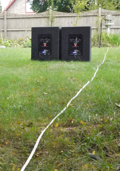
Figure 1
Quantifying this requires a big, open outdoor space in which to set up subwoofers and measurement microphones and make a bunch of noise. What’s that, you say? Use my back yard? Great idea.
We weren’t too keen on moving the house or tool shed as part of this project, so we see some effect from those boundaries on the following measurements. The distance from which we choose to take measurements will have a pretty significant effect on the arrays’ perceived performance as well, for reasons we’ll discover shortly.
I set up a pair of single 18-inch subwoofers in the center of the yard and placed measurement mics twenty feet to the front and rear, which is as far away as I could get without ruining the garden. The two-mic setup, shown in Figure 1 from the perspective of the rear microphone, allows us to see what’s happening both “out front” of the array and “on stage.”
We start by looking at a single sub (Figure 2) and we see why there’s a demand for subwoofer beam-steering in the first place. The black trace shows the front response and the red trace shows the rear. Focusing on the two octaves of most interest to sub performance (31 – 125 Hz), we see that the front and rear response levels are similar.
From this, we can conclude that pointing a sub the other way does very little to steer its output. If we want it to be loud out front and quiet on stage, we’ll have to find another way. (Nerd Note: For visual clarity, all the transfer function traces shown use 1/12 octave averaging, although I normally use 1/24 octave resolution in practice. Temporal averaging was six seconds and the stimulus was band-limited pink noise, which the neighbors loved.)

Figure 2
Going The Distance
Another commonly raised objection to sub steering in general is that rearward rejection comes at the price of decreased output in front. This is true, with qualification. Decreased forward efficiency in sub arrays comes from two main factors.
First, certain array configurations result in delayed and/or out of polarity energy in the forward direction. The severity of this depends on the specifics of the array, which we’ll examine. The other factor is less intuitive: maximum summation from two subwoofers (+6 dB) happens only with a contribution of two equals: two sources meeting at a point in space at equal time, with equal level.
All of the two-element arrays examined here use physical displacement as part of the steering mechanism. In plain English, some of the boxes are placed closer to the audience than others, which creates a level offset and prevents us from ever achieving the full +6 dB. The good news is that level offsets are relative so as we get further from the array, the few feet of displacement matters less and less. (Mr. van Veen calls this “auto-efficiency.”)
Our measurement mics placed 20 feet out will see far more of a level offset than an audience member standing 60 or 70 feet back. To see how big of a deal this really is, we’ll be comparing the forward-going output of each array to the output of a standard side-by-side “broadside” sub array exhibiting the full +6 dB summation, which we’ll call the Gold Standard.
Inline Gradient Array, Non-Inverted
First up is an inline, non-inverted gradient array. (Sometimes this configuration is referred to as an endfire array, although I prefer to reserve that term for arrays consisting of three or more elements in a line. Hold that thought.) Figure 3 shows a side view of the physical configuration: one of the boxes placed closer to the audience.
This array creates a rear cancellation centered on a relatively small frequency range, and the physical spacing of this setup is determined by the frequency we want to cancel.
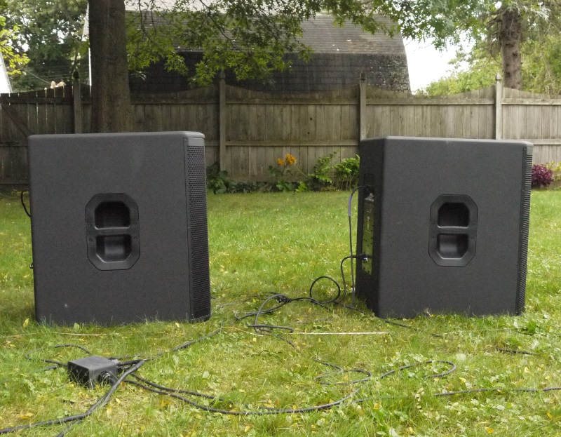
Figure 3
I usually aim for about 65 Hz, right in the middle of the sub range. The two elements should be placed with their acoustic centers spaced a quarter wavelength apart, which for 65 Hz is about 4 feet plus 4 inches (4’/4″). The front box, being closer to the audience, is delayed by the amount of time it takes the output from the rear box to catch up. We can easily calculate that sound waves travel 4’/4” in about 3.8 milliseconds (ms).
In practice, the timings can be slightly higher, since the sound from the rear box has to wrap around the front box, rather than passing straight through it “as the crow flies.” For this reason, performance will be better when delay values are determined with an analyzer rather than a tape measure.
Figure 4 shows the situation in front of the array: the magnitude panel on top shows that the front box (blue trace) is louder because it’s closer to the mic – this is the aforementioned level offset, which will shrink as we move away from the array.
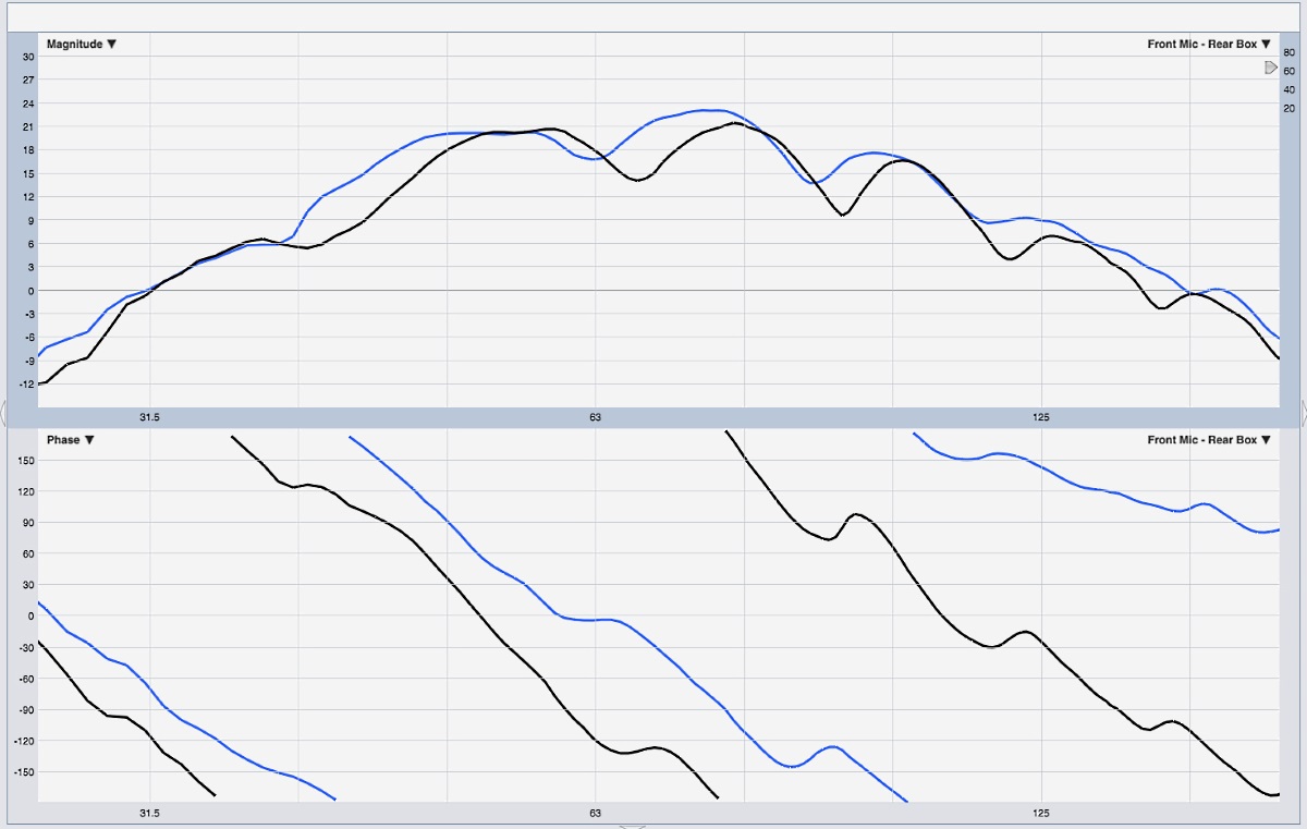
Figure 4
The bottom panel shows the phase response. This isn’t meant to be a dissertation on interpreting fast Fourier transforms (FFTs), so those unfamiliar with decoding phase traces will be well served by this basic relationship: a steeper phase slope means more time offset. The black trace, representing the rear box, has a steeper slope because it’s farther from the mic and so its output takes longer to arrive.
To align this array, no calculations are necessary – just add delay to the front box until its phase trace tilts down to match that of the rear box, which tells us that we’ve got matched arrivals out in front.
In the back of the array, it’s a different story indeed: the output from the rear box arrives first, and the output from the front box is quite late – it’s physically farther away, and it’s electronically delayed. The physical 4’/4” of propagation delay (3.8 ms) adds to the electronic delay (also 3.8 ms) to create a cumulative time offset of 7.6 ms at the rear.
This is where realize the importance of the spacing we chose earlier: 7.6 ms is half a cycle at 65 Hz, meaning the output from the two subs is separated by 180 degrees at this frequency, causing a cancellation. That time offset corresponds to a different phase offset for other frequencies, and since 180 degrees is our “best case scenario” for a deep cancellation, the quality of the rear rejection rapidly decreases above and below 65 Hz.
Figure 5 shows the rear response (red), as well as how the output in front (black trace) compares to our Gold Standard of the full +6 dB that we’d get from a standard broadside arrangement.
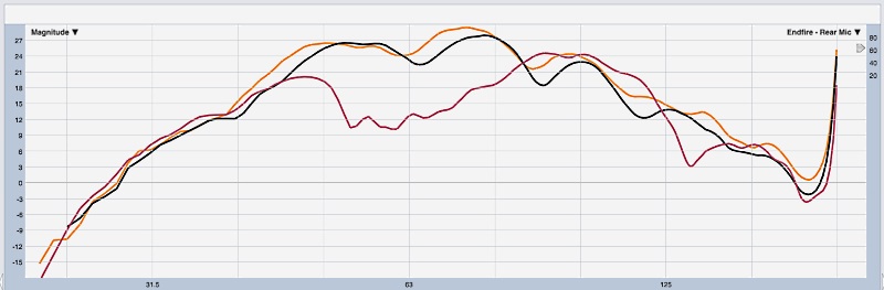
Figure 5
We’ve created a nice bit of rear rejection centered in the 65 Hz region, and… not much else. Outside of that 65 Hz dip, we might as well be standing in front of the array. From our mic position 20 feet out in front, efficiency is within a few dB of Gold and will get even better as we move deeper into the audience area.
We also have a pretty clean output, with only a single, in-polarity arrival out front, so this array configuration has minimal sonic degradation. Unfortunately, there’s little gained in terms of rear rejection, either.
Constructing a larger, four-element endfire array based on the same principle provides more scattered arrivals in the rear and can achieve excellent broadband rear rejection – if you have the subs and the space!
Inline Gradient Array, Inverted
The problem with relying on phase offset to achieve rear cancellation is that it doesn’t hold over frequency. This time, we’ll use polarity, which is frequency-agnostic, to build a rear cancellation that holds throughout the entire frequency range.
The physical configuration is identical to the previous array, however this time it’s rear box, rather than the front, that’s delayed. This array is tuned from the rear – while viewing the response from the rear mic, the upstage box is delayed until its arrival matches that of the front box.
At this point it’s the same array we just explored above, only firing the other way. Then the upstage box is polarity-inverted, turning a rearward summation into a rearward cancellation. The rear-going wave from the front sub is well-cancelled by that of the rear sub. (This is exactly how noise-cancelling headphones work, by the way.)
Figure 6 shows the proper situation in the rear, with the two phase traces 180 degrees apart at all frequencies, indicating an out-of-polarity state.
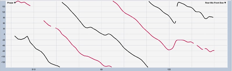
Figure 6
Figure 7 shows the respectable broadband rear rejection achieved as well as the comparison to Gold in the forward direction. Remember that the rear cancellation will improve with distance. A downside of this configuration is worse transient performance – out front, we have late and out-of-polarity energy arriving from the rear box. The comb filtering doesn’t set in until above 100 Hz, but the transients can seem less “punchy.”
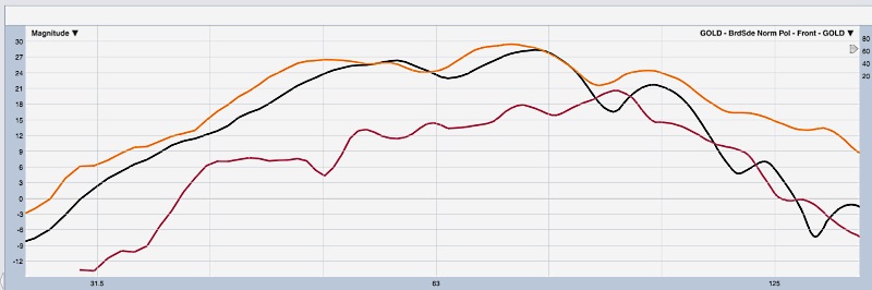
Figure 7
Stacked Gradient Array
Our final stop on this tour involves stacking the two subwoofers on top of each other, with one of the boxes physically reversed. As we’ve discovered, pointing a box the other way does nothing to steer the output, but it’s done here to obtain physical displacement between the drivers – useful if we’re flying a column of them, for example.
The idea is the same as the previous array: the rear-facing box is delayed and then polarity-inverted to cancel the rear-going radiation from the front-facing box. Although the boxes themselves are only about 24 inches deep, the length of the wraparound paths actually approaches that of the inline array, so the timings are similar, and the mechanism still works. Here’s the rub: the rear-facing box has a level advantage at higher frequencies, because they’re no longer omnidirectional, so the level offset between the two boxes increases with frequency (Figure 8).
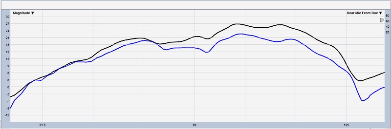
Figure 8
Notice that in the low end of the range, the levels are matched, but by 100 Hz, the rear sub (black) has a clear lead. Some manufacturers recommend a level offset as an attempt at fixing this, but there are two problems: 1) the level offset between the boxes varies over frequency, so gain won’t fix it, and 2) level offsets (or different EQs) mean that one box will go into limiting before the other, leading to “pattern implosion” when the array is working hard and we need the pattern control the most.
For this reason, the rear cancellation achieved by this array is most effective in the LF range where the levels are matched in the rear, shown with the Gold Standard in Figure 9. In the wild, this array type is commonly seen with at least three boxes, alternating front-back-front. As with the previous array, the late and out-of-polarity energy going forward can be cause for concern. Is it a problem? Set up a listening test and decide for yourself.

Figure 9
Wrapping Up
There are other facets of this concept that we don’t have space to delve into here, but I will note that these configurations all need space: since they depend on the wraparound paths to function, they don’t work well when jammed under a stage or against a proscenium.
The question is often raised as to which of these arrays is “best.” The answer depends on the specifics of the situation. Sometimes rear rejection isn’t necessary or even desired. Sometimes it’s paramount. The best outcome is realized by having multiple array types in your “bag of tricks,” understanding the benefits and drawbacks of each, and choosing the most appropriate for each situation.
For more in-depth information, a good starting point is Electro-Voice (electrovoice.com) white paper “Subwoofer Arrays: A Practical Guide” by Jeff Berryman, also available on ProSoundWeb.