Observing the Comb Filter in the Wild

One of the cardinal sins of the average FOH is measuring the PA with both sides on. This sounds perfectly normal to us, because it’s what we’re used to hearing, but the analyzer reveals the truth – the comb filter – if we know where to look.

To illustrate, here are two actual traces measured OnAx to the top boxes of modern line array systems in two different rooms.

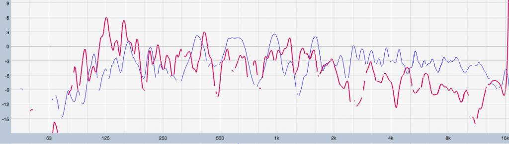
The blue trace is of a system tuned for speech reinforcement, which is why the response is much flatter. These are both somewhat representative of what we can expect this far back in a venue. One of these systems was measured (not by me) with both sides on, and the tech didn’t realize it at the time. Can you tell which?

Many users of dual-channel FFT software seem to prefer viewing the magnitude response only, hiding the phase and coherence traces. This is probably a holdover from the days of RTA, when low-resolution magnitude data was all we had. But by hiding these other traces, we lose any ability to see time-domain issues with the system, as well as the analyzer’s attempt to stop us making decisions based on unreliable data.

If you’re foggy on Coherence, the elevator-pitch version is that it acts as a data quality indicator. Or, basically, “can this data be trusted?” From the Rational Acoustics Smaart v8 user guide [pdf]:

Coherence is a statistical estimation of the causality or linearity between the reference and measurement signals in a transfer function measurement. Coherence does a good job of detecting contamination of the measurement signal by unrelated signals such as background noise and reverberation, and it is sensitive to timing mismatches as well. We use it in Smaart to gauge the quality of transfer function measurement data, frequency by frequency, in real time. […] The coherence calculation essentially asks the question, “How confident can we be that what we are seeing in the measurement signal at this frequency was caused by the reference signal?”

Showing the coherence and the phase traces gives us the whole story:

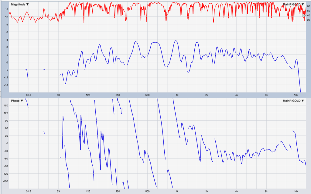
The coherence trace shows a regularly spaced series of peaks and dips. When I say “regularly spaced,” I mean “getting closer together as frequency rises” because we usually view frequency-domain information on a logarithmic axis. This is the analyzer letting us know something is suspect. At these frequencies, the two hangs are destructively interfering, resulting in low coherence that corresponds with the deep dips in the magnitude trace. Also, check out the phase trace at the same points: the little jaggies are indicative of a summed phase response that results when the analyzer is trying to decide between two sources of timing information.

By contrast, here’s the full data for the other (single-sided) measurement:

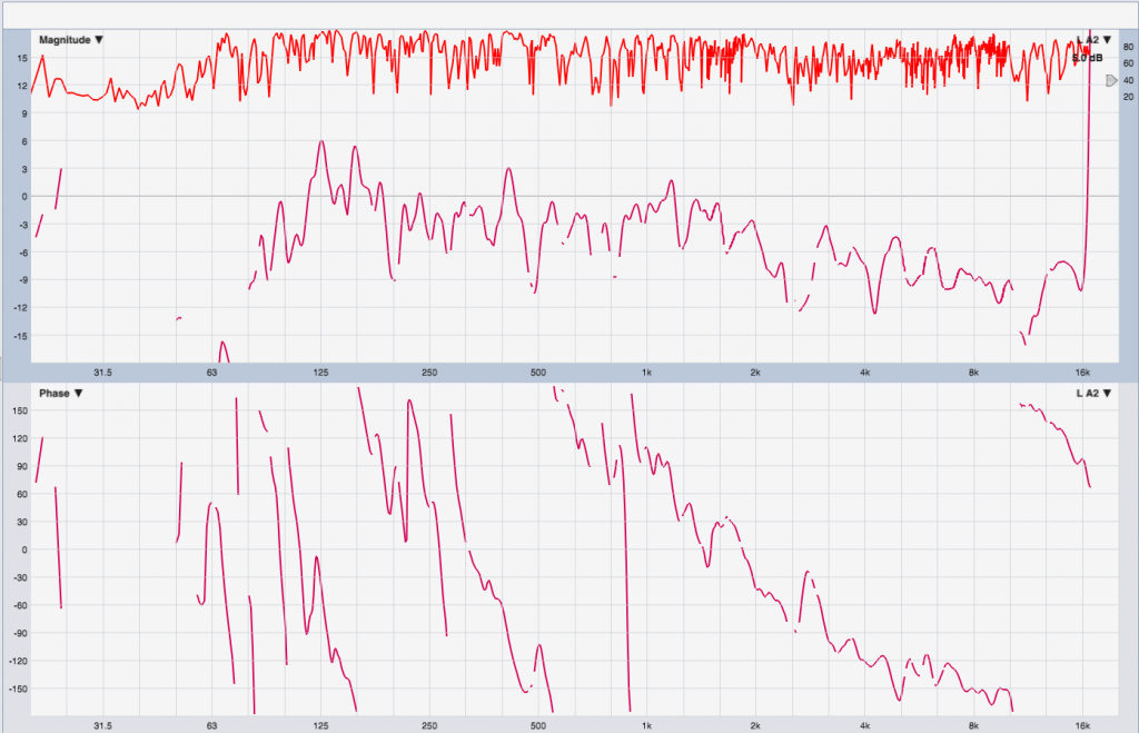
We still see dips in the coherence trace because we’re so far back in the room (about 65 ms) but they’re definitely not caused by a comb filter this time. No regular spacing, and no corresponding phase jaggies.

So we need to learn how to recognize the comb filter problem in the wild so we don’t go in with 22 PEQ filters and try to fix something that’s not broken in the first place (I see this more often than you might think). Let’s view the same comb filtered response on a linear frequency axis:

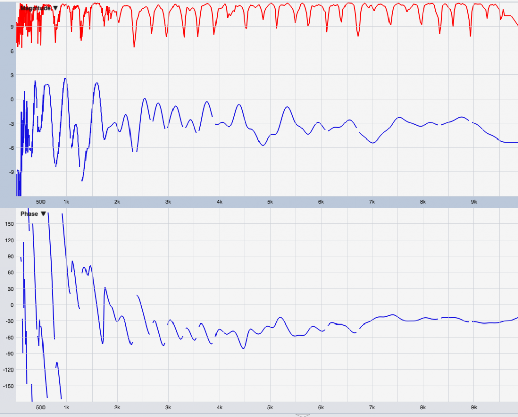
Plain as day. I’m not suggesting that you work with a linear frequency axis, as it bears very little resemblance to what we hear (half the audible spectrum is compressed into 10% of the plot) but it readily reveals time domain issues. Now looking back at the same data on the log axis, it should be a bit easier to see.

Just for fun, let’s figure out how far off the mic was. Zooming in a bit reveals that the response dips are spaced at about 290 Hz, meaning the filter is completing a full cycle (360°) in 290 Hz. Since T = 1/f, that corresponds to a time offset of about 3.5 ms, which means a path length difference of about 3.9 feet.

However, a lot of system techs train themselves to think of distance in terms of milliseconds, as it eliminates the mental calculation and keeps things in terms that are readily related to system optimization workflow. Eventually, rather than having a mic placement 80 feet back in the room, we think of the mic placement as 71 ms back in the room, which corresponds directly to the analyzer’s compensation delay settings.