Exploring Large-System Level Variance Compromises

Our heroes find themselves in a larger reverberant space (an armory, actually) which is, of course, the best environment for events requiring speech intelligibility. PA is twelve dual-15 boxes per side with a sub “mono block” on the ground front and center. The optimization you see here was masterminded by my friend David, whom I always enjoy working with because we see eye to eye on most areas of approach, and I think he did a great job with this.

Ground Plane vs Ear Height Measurement

Folks seem to be very scared of the ground bounce. I’ve written a bit about dealing with it in the past but it’s often a fact of life – both for our measurement and for our audience’s ears. To quantify the issue on a reflective wooden floor, the blue trace shows the ear-height measurement, and the pink trace shows the measurement obtained by placing the mic on the floor directly below. (It’s best to still leave your mic stand near the mic when doing this so people don’t drive forklifts over it.)

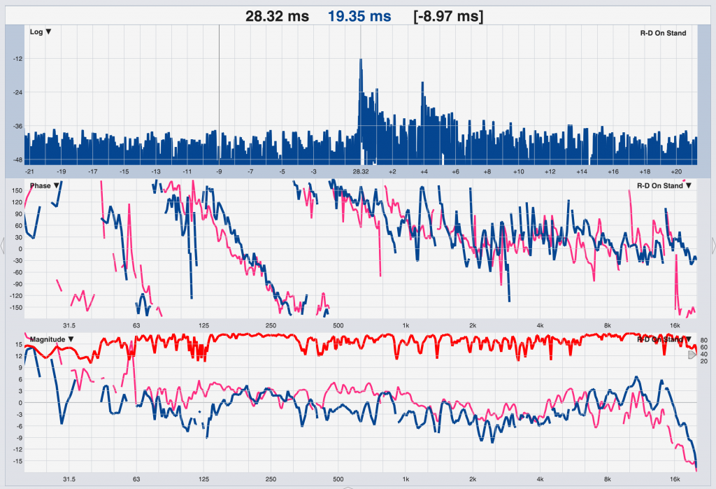
I don’t always include the Live Impulse Response view in screenshots, but it’s an important piece of the puzzle here. I’ve increased the size of the Live IR pane for clarity (Options>Transfer Function>Proportional Panes). The primary arrival shows in the center of the pane at 28.32ms, with the floor bounce clearly arriving as a second peak almost exactly 4ms later.

Note the far jaggier phase trace (middle pane) particularly above 1k. That’s the analyzer trying to deal with two conflicting phase values per frequency. Any time we see these “mini wraps” we should be looking for a time-domain issue.

Below that, in the magnitude response, we see the first few dips of a comb filter. (Why aren’t the peaks +6 dB above the floor measurement? Two reasons – the second arrival is not of equal level, so we achieve neither deep cancellation nor perfect +6 dB summation. This is evident on the IR as a second peak that’s not as tall. Also, the ground plane measurement is technically +6 dB summation at all frequencies.)

The second arrival at about 4ms means a full cycle behind at about 250 Hz, where we indeed see a peak. 125 Hz is seeing an arrival 180° late (half cycle, most cancellation) and we do see a 12 dB deep dip in the response at 125 Hz. This won’t go away with EQ (or auto-EQ…) and is a good example of how making tonal decisions without time-domain data can be problematic.

Front To Back Variance

I am probably a bit more stubborn than many of my peers when it comes to front-to-back level variance, in that I spend quite a large percentage of my optimization time trying to reduce the front to back level difference as much as practical.

“Practical” is an important word here. Stage wash does fall off with distance, so if it’s a loud stage, you will want some more gas out of the PA down front so folks can hear the show properly. The elephant in the arena, though, is that subs are far more likely to fall off at the usual rate over distance unless we get to do something fancy with them in the air, and our options to reduce that rate are usually quite limited, so having your mains perfectly level-matched all the way back will probably mean that the spectral balance shifts dramatically against the subs underneath, and that’s generally not a trade I’m willing to take. So it requires some consideration. The goal of “same show everywhere” means considering both spectral and level variance, and you make a judgement call.

But when we can do it, it’s quite rewarding to actually pull it off. Here’s what it looks like in a 700 seat theater I mix regularly, with measurements taken at four locations from front to back of the audience area:

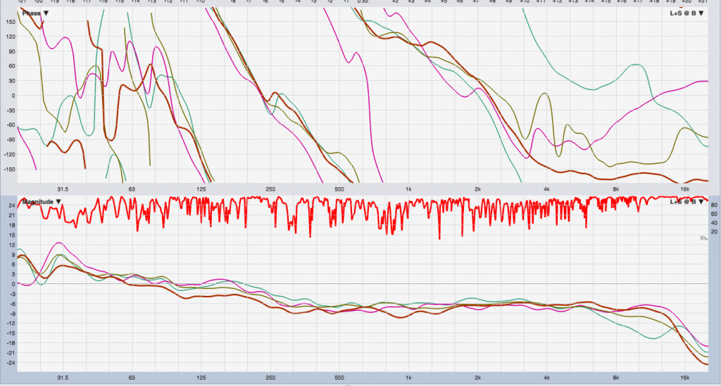
I focus efforts above 1 kHz and particularly on the intelligibility region from 2k – 4k where our ears are most sensitive and where much of our loudness perception is driven – and where per-zone EQ or level is particularly effective. Below 1 kHz, our options start to shrink, as the array’s energy is morphing into a single “beam” that doesn’t really respond to shading or EQ on individual boxes. With longer lines, chasing a few dB of variance at 350 Hz requires something sophisticated like Meyer’s all-pass-based Low Mid Beam Control, and is quite low on the priority list in my opinion. (It can be done by hand but it’s extremely hard to quantify and there are serious consequences for screwing it up, so I generally don’t go there.)

How well does this approach hold up on a larger scale? This 12-box hang was driven in four zones of three boxes each. We took ground-plane measurements of the entire array as close to “ONAX” of each zone as possible. The perspective is kind of weird but this is the only photo I had clearly showing all four placements.

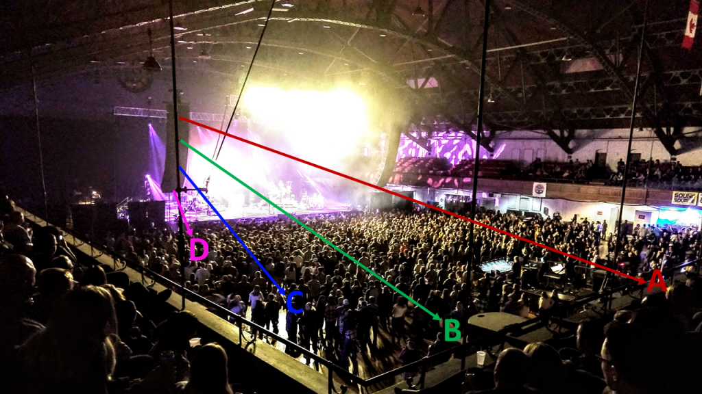
For the (very shallow) balcony (A, red) I set the mic flat against the flat wooden cupholder edge of the balcony, which provides the closest approximation to the true floor placement of the other measurements. We will see the effects of that placement in the measurement.

The top boxes are throwing about 95 feet, and the bottom boxes are throwing about 12 feet, a Range Ratio of 8:1 or 18 dB. Here are the measurements color coded to match the photo:

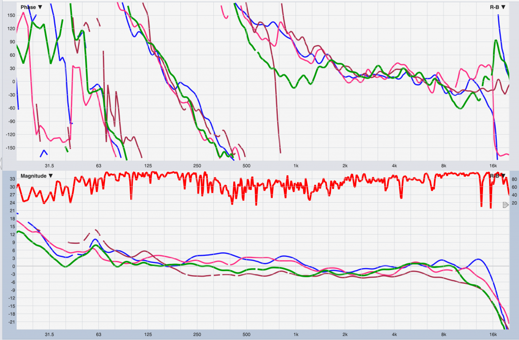
Between 250 and about 1 kHz, the radiation is more or less aimed from the geometric center of the array, which is why the mid-frequency lobe is loudest around position C (blue). It’s also high in front (D, Pink) probably due to sheer proximity. The balcony is the farthest throw, and so lowest in overall level, but we can see what I assume to be the combined effects of mic placement against a smaller boundary (less MF boost), and proximity to the back wall and probably balcony face (LF runup below 125), in addition to the telltale effects of air absorption above 6k. This could be brought back with EQ if desired, but very carefully as it will likely change come showtime. For that reason it tends to be a decision I will make by ear during the show. This is another area where complete elimination can seem psychologically unnatural (people don’t expect something that looks 100 feet away to sound like it’s up your nose) so I will often aim for reduction, rather than elimination, of the variance up this high.

In the critical 2k – 4k octave we are quite well balanced indeed, and the perception walking around during the show was that it did indeed sound pretty darn consistent.  An alternative approach here is to swing the pendulum more towards spectral consistency, take the varying midrange response as a given, and work with the HF to match. This is much harder to predict ahead of time and will probably take longer in the room. Again, the show dictates the approach here.

The biggest spatial variation by far was the sub coverage (not shown above) falling off on the sides of the room, to be expected given the deployment, which in this case was requested by the production.

Walking the space, we were quite pleased with the HF consistency despite the rather aggressive shading it took to achieve it. I try to eliminate as much of the front-back level variance as possible via splay angles, and rigging restrictions forced David’s hand in that regard here. However, 2° at the top over 10° at the bottom can be expected to provide a few dB shy of the theoretical 20log(2/10) = -14 dB of HF level reduction at the bottom (in practice this comes out to about 11 dB).

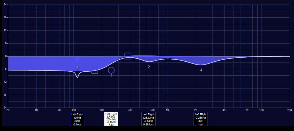
We ended up with the bottom boxes shaded down by 6 or 7 dB, which actually brings us almost perfectly back to negating the theoretical 18 dB Range Ratio. (Top to bottom zone shading was 0 dB, -2 dB, -4 dB, -7dB). The numbers are a little scary but I can’t argue with the results. Concerns about LF headroom are allayed by the fact that over 6 dB had already been pulled out via a low shelf, creating more LF headroom than needed.

Note that this isn’t always the case, and you can get yourself into trouble with that much shading if you’re low on headroom to begin with and you expect the show to run the PA to its limits. Having certain boxes hitting the limiters sooner than others can be a problem in that case – but it’s worse if the top boxes hit limiting that the FOH engineer can’t hear, so in general it’s safer to take the bottom boxes down some. It can also cause some interesting imaging effects but if you’re standing directly under the array, my feeling is “that train has sailed,” as Austin Powers would say.

How much LF headroom was lost?

• The unshaded case of four zones each operating at unity is 0 dB + 0 dB + 0 dB + 0 dB = 12 dB (two doublings).

• In linear, that’s 1+1+1+1 = 4.

• If we shade as above, that becomes (0 dB) + (-2 dB) + (-4 dB) + (-7 dB)

• which in linear math is 1 + 0.8 + 0.63 +0.45 = 2.9.

• From there, we take the ratio of the unshaded case vs the shaded case by 20log(2.9/4) = -2.8 dB.

There are some shows where this might be valuable headroom, in which case less shading is advisable. Another option is to use a high-shelf filter to reduce only HF response while leaving the LF at full power. (Do not try to do this by turning down HF amp channels.)

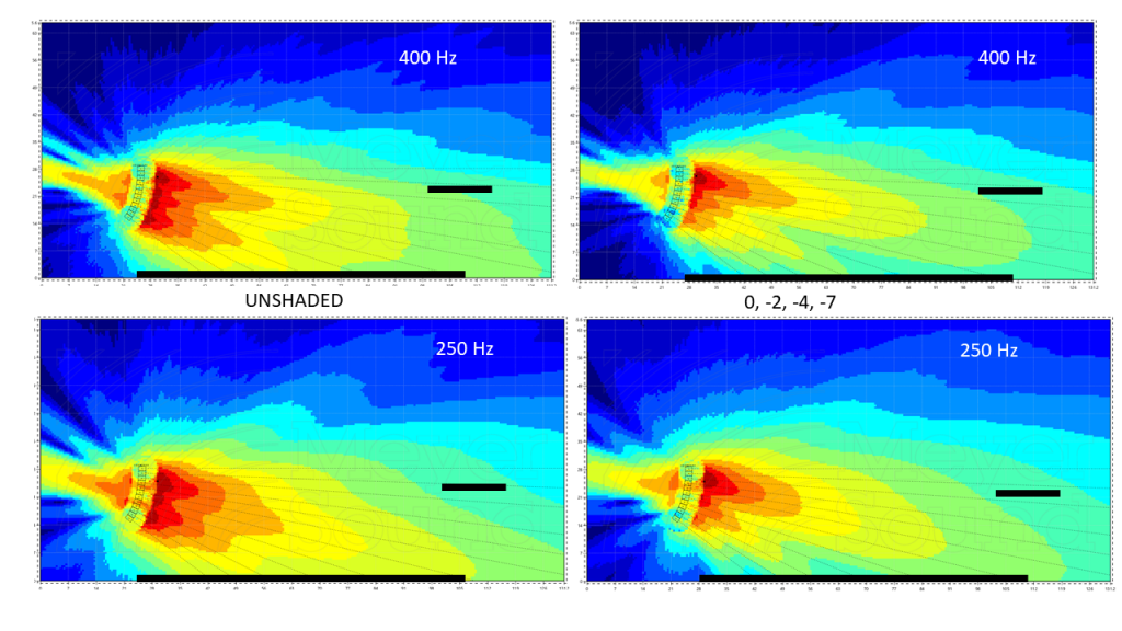
To address concerns about the effects of shading the low-mid beam directionality: A quick prediction of a similar-sized array at a similar height with similar angles in a similar sized-venue shows that it argulably increases uniformity by sending more lo-mid energy towards the top of the array, and thus the coverage shape at these frequencies is possibly a better match for the HF shape. In my book, that’s a step forward in this context. If not, I’d look towards high shelving rather than gain shading – or reworking the splay angles if that’s an option.

I think it is fair to say that this is an example of how a good understanding of the tradeoffs involved with an optimization decision can help you decide whether or not it’s a good fit for the goals of the project. And if we don’t get it right, that’s more info and context for next time.